The CLTDSCLCLF Cooling Load Calculation Method [PDF]

Zitiervorschau

This paper has been downloaded from the Building and Environmental Thermal Systems Research Group at Oklahoma State University (www.hvac.okstate.edu) The correct citation for the paper is: Spitler, J.D., F.C. McQuiston, K. Lindsey. 1993. The CLTD/SCL/CLF Cooling Load Calculation Method, ASHRAE Transactions. 99(1): 183-192. Reprinted by permission from ASHRAE Transactions (Vol. #99, Part 1, pp. 183-192). © 1993 American Society of Heating, Refrigerating and Air-Conditioning Engineers, Inc.

3638 RP-626

THE CLTD/SCL/CLFCOOLING LOAD CALCULATIONMETHOD J.D. Spitler, Ph.D., P.E. Member ASHRAE

F.C. McQuiston,Ph.D., P.E. Fellow ASHRAE

ABSTRACT This paper describes a thorough revision of the cooling load temperature dfference / cooling load factor (CLTD/CLF) method. The major revisions made to the original CLTD/CLF method are: 1.

The calculation procedure for cooling loads due to solar radiation transmitted through fenestration was revised with the introduction of a new factor, the solar cooling load (S C L ),which is more accurate and easier to use. Previously, cooling loads due to solar radiation transmitted throughfenestration were somewhat inaccu rate when a latitude/month combination other than 40 °N/July 21 was used. 2. The new weighting factor and conduction transfer function coefficient data developed by ASHRAE RP-472 were used to generate new CLTD and CLF data. A limited data set is available in printed form, and software has been developed to generate custom CLTD and CLF tables. Previously, the limited number ofzone types used to generate the original CLTD/CLF data resulted in sign jfi cant error for some zones.

INTRODUCTION The cooling load temperature difference I cooling load factor (CLTD/CLF) method has been a popular method for performing cooling load calculations since the publication of ASHRAE GRP-158, the Cooling and Heating Load Calculation Manual (ASHRAE 1979). Originally developed as a hand calculation technique, it was constrained to use some approximations that resulted in significant inaccuracies under some conditions. ASHRAE Research Project 359, completed in 1984 (Sowell and Chiles 1985), revealed some limitations of the applicability of the CLTD!CLF factors given in GRP-158. The research revealed that factors not taken into account in the original work could significantly affect the results. ASHRAE Research Project 472, completed in 1988 (Sowell 1988a, 1988h, 1988c; Harris and McQuiston 1988) resulted in new categorization schemes for walls, roofs, and

K.L. Lindsey

zones, as well as normalized CTF coefficients and weight ing factors that corresponded to the categorization schemes. The data base of weighting factors developed was much too large to be used in printed form. However, the widespread availability of personal computers allows the possibility of distributing the data on diskette. The results of ASHRAE Research Projects 359 and 472 represented the possibility of substantial improvement in the CLTD/CLF load calculation method and data compared to GRP-158. Other research that impacted load calculation techniques or data had also been published since the development of GRP-158—particularly in the areas of solar radiation, appliance heat gains, and material properties. Furthermore, access of engineers to personal computers had drastically improved since 1979, which made the use of more sophisticated load calculation techniques possible. The above factors taken together suggested the need for a new load calculation manual. ASHRAE Research Project 626 focused on three areas: revision of the load calculation manual, revision of the CLTD/CLF method, and develop ment of software that could access the data developed by RP-472. This paper describes the revised CLTD/CLF method, now known as the CLTD/SCL/CLF method. A companion paper (Spitler et al. 1993) describes the rest of the load calculation manual. A third paper describes the software developed to access the RP-472 data (Falconer et al. 1993).

BACKGROUND C L T D 1 C LM F ethod The current cooling load temperature difference I cooling load factor (CLTD/CLF) method described in GRP 158 (ASHRAB 1979) is based on work done by Rudoy and Duran (1975). This method was developed as a hand calcu lation method, which would use tabulated CLTD and CLF values. The tabulated CLTD and CLF data were calculated using the transfer function method, which yielded cooling loads for standard environmental conditions and zone types. The cooling loads were then normalized, as described below, so that the designer could calculate the cooling load

Jeffrey D. Spitler is an assistant professor, Faye C. MeQuiston is a professoremeritus, and Kirk L. Lindsey is a graduate student in the School of Mechanical and Aerospace Engineeringat Oklahoma State University, Stiliwater.

ASH RAETransactions:Research

183

for each hour with a simple multiplication. The cooling loads for each component were then summed to obtain the total zone cooling load. Walls and Roofs The transfer function method (TFM) was used to compute cooling loads for 36 types of roofs and 96 different wall constructions. These cooling loads corre spond to the heat gain caused by outdoor air temperature and solar radiation under a set of standard conditions, which included a latitude of 4ON, date of July 21, maxi mum outdoor temperature of 95°F, daily temperature range of 21°F, and an inside design temperature of 78°F. Fur thermore, a single standard zone type was used. Hourly cooling loads for each hour were converted to cooling load temperature difference (CLTD) values by dividing by the roof or wall area and the overall heat transfer coefficient. The cooling load could be calculated for any wall or roof by the following relation (1) q = U A CLTD where q UA CLTD

=

=

cooling load, Btu/h; overall heat transfer coefficient, Btu/hft2 °F; area, ft2 equivalent temperature difference, °F.

CLTDs were calculated for 96 types of walls for a medium type of zone construction. The CLTDs were analyzed for similarity in profile and peak value. Walls were then grouped into seven different categories, and CLTDs were tabulated for eight facing directions. CLTDs were calculated for 36 types of roofs. GRP 158 grouped the roofs into 13 categories with suspended ceilings and 13 without suspended ceilings, making 26 categories in all. The following equation was given to adjust for other latitudes and months and other indoor and outdoor design temperatures: (CLTD + LM) CLTD (2) K + (78—TR) + (T0-85)

3.

if a wall or roof does not match one of thegroups listed (e.g., for each increase of 7 in R-value above that of the wall structure in the listed group, move up one group if insulation is on the interior of the structure and two groups if on the exterior.) The inaccuracy of correcting for other months and latitudes can be significant.

Fenestration To find the cooling load due to fenestra tion, the heat gain was divided into radiant and conductive portions. The cooling load due to conduction was calculated using the same relation used for roofs and walls (Equation 1). CLTDs for windows were listed for standard condi tions, and a relation was provided to correct for outdoor daily average temperatures other than 85°F and indoor temperatures other than 78°F. No latitude-month correction was provided, but the conductive load from fenestration is such a small portion of the overall load that this was deemed negligible. To find the radiant portion of the cooling load, the solar heat gain for each hour through a reference glazing material (double-strength, 1/8 in. sheet glass) was calculated for different fenestration orientations using the ASHRAE clear sky model. Using the weighting factor equation, cooling loads corresponding to these heat gains were calculated for light, medium, and heavy zone constructions without interior shading and for zones with interior shading. A cooling load factor (CLF) was derived for each hour of the day so that the cooling load for that hour could be found by multiplying the maximum solar heat gain for the day by the hourly CLF as follows: (3) Q = SHGF . SC . CLF A where

Q SHGF CLF

=

SC

=

A

=

=

where LM

=

K

=

=

latitude month correction factor, found in a table; color adjustment factor, applied after latitude month correction; room temperature, OF; outdoor temperature, °F.

The drawbacks with the original CLTD method for walls and roofs are as follows: 1. The wall and roof groups don’t cover the range of possible constructions well. 2. Complicated and questionable adjustments are required 184

cooling load for reference glazing system, Btufh; maximum solar heat gain factor, Btu/h; cooling load factor, ratio cooling load to maximum solar heat gain; solar heat gain of fenestration system solar heat gain of reference glass area of fenestration, ft2 .

CLFs were tabulated for July 21 at 40 deg north latitude. These CLFs were considered to be representative of all summer months (May through September) at all northern latitudes. It was presumed that the variation in solar heat gain for other latitudes and dates could be ade quately accounted for using SHGFJ,, which was tabulated for all directions, months, and northern latitudes from 0 to 60 deg. The cooling load at a particular latitude and month was then found by multiplying the SHGF,, for that month and latitude by the CLF calculated for July at 40 deg north. Normalizing the solar heat gain in this manner resulted in what was probably the most serious error in the CLTD/ ASH R AE Transactions:Research

CLF method. The tabulated CLFs could be significantly in error for other dates and latitudes. These errors were most severe for off-peak hours. This error was particularly noticeable near sunrise and sunset for latitude/month combinations that had significantly different sunrise/sunset times than 4ON, July 21. People, Lights, and Equipment For people, lights, and equipment, the hourly heat gains are specified by the designer. The cooling load depends on the magnitude of the heat gain for each hour and the thermal response of the zone. For people, lights, and equipment, the weighting factor equation was used to determine the cooling load for a unit heat gain with various schedules (on two hours, on four hours, etc.). Since a unit heat gain is used, the cooling load factor (CLF) is simply the cooling load. The designer then uses the following equation to determine the hourly cooling load:

Q

=

q 5 CLF

+

q1

(4 )

where

Q

= =

q,

=

cooling load, Btu/h; sensible heat gain, Btufh; latent heat gain, Btu/h.

Cooling load factors for people and equipment were determined using a single medium-weight zone. Cooling load factors for lighting were determined using several zone types, light fixture types, and ventilation schemes.

ASHRAERP-472 / S ow ell The main reason for the limited number of zone types available in the original CLTD/CLF method was the limited amount of weighting factor data available at the time the CLTD and CLF tables were tabulated. Following their publication, it was noticed that for some cases the resulting loads could be significantly in error. An ASHRAE research project, RP-359 (Sowell and Chiles 1985), highlighted the significant and complex effects that various zonal parame ters could have on zone response. This, in turn, led to another ASHRAE research project, RP-472 (Sowell 1988a, 1988b, 1988c; Harris and McQuiston 1988), which exhaust ively analyzed the effect of 14 separate zone parameters on zone response. Three papers published by Sowell detail the methods used to classify and group 200,640 parametric zones. The first paper (Sowell 1988a) describes the methodology used to calculate the weighting factors with a modified version of DOE 2.lc. The second paper (Sowell 1988b) describes the verification of the weighting factor calculation methodology. The third paper (Sowell 1988c) describes the procedure used to categorize the zones into groups with similar zone responses for each of the four different heat gain categories: solar, conduction, lighting, and people/equipment. The resulting set of grouped weighting factors was still ASHRAETransactions:Research

rather large and certainly would be too unwieldy to use in printed form. Therefore, one part of ASHRAE RP-626 involved the development of a transportable data base of weighting factors and access software in C and FORTRAN. This software is described in a companion paper (Falconer et al. 1993). ASHRAE RP-472 I M cQ u isto na nd H arris To use the CLTD method for walls and roofs, one had to determine which wall or roof type a particular surface matched. To do this, the overall conductance and thermal mass were determined for the surface in question and compared to those of the tabulated surface types. If a surface did not exactly match a listed surface type, a complicated set of instructions were followed to pick the best match. This method was tedious to apply and its accuracy was questionable under certain conditions. Harris and McQuiston (1988) performed a study to devise a method for grouping walls and roofs with similar transient heat transfer characteristics in order to obtain a compact set of conduction transfer function (CTF) coeffi cients that would cover a broad range of constructions. The walls and roofs were classified on the basis of their thermal response characteristics, particularly the time lag and amplitude reduction for a sinusoidal driving function. The amplitude ratios and time lags were studied for 2,600 walls and 500 roofs. The walls and roofs were grouped on the basis of these thermal characteristics into 41 groups of walls and 42 groups of roofs with a set of CTF coefficients assigned to each group. Correlation methods were used to find correlations between the amplitude ratio and time lag and the wall or roof’s physical properties or geometry. Important grouping parameters for walls were found to be 1. principal wall material (the most massive material in the wall), 2. the material with which the principal material is combined (such as gypsum, etc.), 3. the R-value of the wall, and 4. mass placement with respect to insulation (mass in, mass out, or integral mass). Important grouping parameters for roofs were found to be 1. principal roof material (the most massive material in the roof), 2. the R-value of the roof, 3. mass placement with respect to insulation (mass in, mass out, or integral mass), and 4. presence or absence of a suspended ceiling. Using these parameters, one can determine to which of the groups a particular waIl or roof will belong. Each group was assigned a unique set of conduction transfer function (CTF) coefficients so as to produce conservative results.

185

These coefficients are to be used in the CTF equation to calculate a representative heat gain for any wall or roof in that particular group.

O BJEC TIVES With respect to the CLTD/CLF method, the goals of this project were to 1.

2.

improve the accuracy of the CLTD/CLF method, talcing advantage of advances in the state of the art made by RP-472 and other research, and provide a method that could be used without a comput er for engineers who do not make use of a computer.

The calculation of cooling loads due to solar heat gain through fenestration is flawed due to the methodology employed to normalize the data 2. The effects of zone response are inadequately account ed for, with either a single zone type or a few zone types for each type of heat gain. 1.

The revised methodology, described below, resolves the two problems as follows: 1.

To some degree, these goals conflict. Only a limited amount of improvement to the method can be made without relying on either a computer or an impractically unwieldy set of printed tables. •I’h isconflict was resolved by provid ing three different ways the method may be used: 1.

Solely as a manual method, using a small set of printed tables in the new manual. Printed tables were designed and published in the manual for quick and convenient hand calculations covering most common constructions with as little loss in accuracy as possible. It was decided to design the printed tables so that they could be used if needed as a stand-alone reference for cooling load calculations during the month of July. The printed tables can also be used alone to calculate cooling loads for northern latitudes from 20 to 50 degrees by using interpolation or extrapolation of supplied tabular results. 2. Primarily as a manual method, using the computer only to generate a set of tables equivalent to the printed tables, except for latitude and month. The computer program CLTDTAB can generate tables identical to the printed tables in the manual for any month and latitude specified by the user. A one-time run of the computer program will eliminate the need for interpolation due to different latitudes and allow hand cooling load calcula tions for months other than July. 3. Primarily as a computer method, using the computer program CLTDTAB, Zone Specific option, to generate a set of tables for a specific zone, latitude, and month. The program will generate tables to facilitate the cooling load calculation for any zone with any roof type and wall type, rigorously following the transfer function method. Tables can be generated for any month and latitude of the user’s choosing.

METHODOLOGY The inaccuracies of the original CLTD/CLF method discussed above can be condensed into two fundamental problems: 186

The cooling loads due to solar heat gain through fenes tration are now calculated differently. A new factor is introduced, the solar cooling load (SCL). Although it would have been possible to fix the old method by also tabulating CLFs as a function of month and latitude, and thereby retaining the same equation, it would have involved a totally unnecessary step—multiplying the SHG FM JCby the CLF, both of which would be func tions of latitude and month. Instead, the SCL takes into account both the solar heat gain and the zone response for any latitude/month combination. It is applied with the following equation: (5) = SCL ‘SC ‘A .

Q

Accordingly, the name of the method has been revised, and it is now called the CLTD/SCL/CLF method. 2.

The zone response can now be accounted for in a more accurate manner, using the weighting factors developed in ASHRAE RP-472. The only limit is the mode of operation in which the designer chooses to work. If the computer-oriented mode (number 3 in the “Objec tives” section) is used, the effects of zone response can be accounted for with approximately the same accuracy as the transfer function method.’ If one of the two manual modes (numbers 1 and 2 in the “Objectives” section) are used, some accuracy is given up in order that the data be reduced to a reasonable number of printed tables.

The methodology used to develop the new CLTD/ SCL/CLF data can be broken into several sections, which follow. The general methodology is used to compute the CLTD/SCL/CLF data, regardless of whether it is eventually put into a set of printed tables or produced at the user’s request by a computer program. The printed tables require some further analysis to choose the zone or zones used for each table. The computer software is described in a companion paper, (Falconer et al. 1993). It is also described in considerably more depth by Lindsey (1991). General Methodology for DevelopingTable Data In capsule, the general methodology can be described as using the transfer function method to determine the cooling loads for a given heat gain type and then nornializ

A S HR A E T ra n s ac tio ns R :e se a rch

ing the load to yield either CLTD or CLF or SCL. A brief description of the methodology follows. For more complete details, see the description of the transfer function method given by McQuiston and Spitler (1992) or the detailed description of the table development given by Lindsey (1991). Solar Irradiation The first step in the analysis is the calculation of solar irradiation, which, in turn, is used to determine sol-air temperatures for opaque surfaces or solar heat gain factors (SHGF) for fenestration. The method used for calculating the solar irradiation is similar to the standard one presented in the 1989 ASHRAE Handbook—Fundamen tals ,“Fenestration” chapter (ASHRAE 1989). It is, in fact, as described by McQuiston and Spitler (1992) to mo1ified compute the transmitted and absorbed components of solar heat gain separately. In addition, the ASHRAE clear sky model uses revised A, B, and C coefficients as recommend ed by Machler and Iqbal (1985). Heat Gain for Walls and Roofs Once the solar irradiation has been calculated, the heat gain for a wall or roof can be calculated using the sol-air temperature (tj, which is the temperature the outside air would have to be to cause the same heat gain to the inside surface as that caused by the outdoor air temperature and solar radiation combined. It is defined by the following equation: (6) = + (cXF)/h0 to + (aXI,)/h0

=

=

‘Ir

I, =

c F

= =

The conduction transfer function coefficients developed by Harris and McQuiston (1988) were used in the conduc tion transfer function equation to calculate thfe heat gain for any hour () due to walls or roofs as follows: q0

=

A[

b(t00_,)

—

d{(q)IA}

—

ç

c0j

(7)

where q0 0

=

U

A 0 0 n

= =

= = = =

heat gain through wall, roof, partition, etc., Btu/h, at calculation hour 0 ; indoor surface area of a wall or roof, ft2 time, h; time interval, h; summation index (each summation has as many terms as there are non-zero values of

ASHRAETransactions:Research

t,cosjO +

=

2 t/(J÷2)

(8)

radiation directly striking surface, Btu/lrft2 angle of incidence; diffuse radiation reflected from ground and sky, Btufhft2 coefficients for radiation transmission through DSA glass.

The radiation absorbed by the glass the following formula: ‘DY.

acosjO

+ ‘d

(Jab)

is calculated with

2 a / ( j 2)

(9)

+

with a

=

coefficients for radiation absorption by DSA glass.

Only a fraction of the energy absorbed by the glass enters the zone; the rest is convected and radiated to the outside. So the heat gain to the zone due to radiation absorbed by the window (Ii,,)is calculated as follows: (10) IIfl N , 1ab with N,

=

—

where

=

outside air temperature, °F; absorptance of surface; total radiation incident on surface, Btu!hft2 outside convective and radiative heat transfer coefficient, Btu/hft2 OF; emittance of surface; difference between the long-wavelength radiation incident on the surface from the sky and the radiation emitted by a black body at the outdoor air temperature, B tm ’h ft2.

the coefficients); no, °F; sol-air temperature at time U constant indoor room temperature, °F; conduction transfer function coefficients.

Equation 7 must be solved iteratively because the heat flux history terms on the right-hand side are not known beforehand when analyzing a 24-hour time period. Initially, the heat flux history terms are assumed to be zero, and Equation 7 is calculated for successive 24-hour periods until convergence is reached. At that time, the results are independent of the values assumed initially. Heat Gain for Fenestration Heat gain to a zone due to windows is broken into two parts, the radiation transmit ted through the glass (T a )and the fraction of the radiation absorbed by the glass that enters the zone, ‘•m. The heat gain due to radiation transmitted through the glass is calculated as follows:

where =

=

tcO.r

=

the inward flowing fraction of absorbed radiation.

The inward-flowing fraction is calculated by neglecting the glass resistance: (11) JV = h,/(h0 + h 1 ) where

187

=

h0

=

inside heat transfer coefficient, 1.46 Btu/lvfi2°F; outside heat transfer coefficient, 4.0 Btufhft2°F.

Conversion of Heat Gain to Cooling Load Once the heat gain has been calculated, whether from walls, roofs, windows, lights, or people, the relation to convert the heat gain to cooling load is the same, with only the coefficients (weighting factors) different. Weighting factors are used to calculate the zone cooling load at time 0, Q 0based on past loads and current and past heat gains using = v 0 q 0 + v1q0 + w1Q08 w2Q0 (12) —

each wall and roof group by dividing the hourly cooling load per square foot for the surface by the overall U-value for that surface. The hourly SCL values are the hourly cooling load values for the reference glazing system for the latitude and month listed and are obtained by adding the cooling load due to the transmitted portion of the solar energy to the inward-flowing fraction of the solar energy absorbed by the reference glazing system. CLF values are simply the cooling load due to a unit heat gain from people, equipment, or lights.

—

where ô =

V1

and w 1

q0

= =

time interval, cooling load at time t, weighting factors, heat gain at time 0.

Previous cooling loads and heat gains are initially assumed to be zero, and calculations are performed in an iterative manner until the results for a 24-hour cycle converge. Calculation of CLTD, SCL, and CLF Values After the cooling loads have been determined, the CLTD, SCL, and CLF can be easily calculated. CLTD are calculated for

Printed Tables Development of a set of printed tables for use with the CLTD/SCL/CLF method inevitably involves a compromise between accuracy and the number of pages required for tables. A complete set (all zone groups) of just the SCL tables for one latitude and one month would require approx imately 22,000 pages to print! A more practical approach, of course, is computer-based table-generation software, which can easily create a set of zone-specific tables. In some cases, however, it may be desirable to work from the set of printed tables contained in the load calcula tion manual. In order to produce a set of printed tables suitable for use in the load calculation manual, several steps had to be taken:

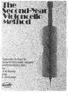
TA B LE1 Zone P aram eterLevelsU sedin D evelopingP rintedTables Parameter

Meaning

Levelsconsiclcrcd

1

ZG

Zone geometty

lOOft.x20ft., l5ftx lSft.

2

ZH

Zone height

8 ft, 10 ft.

3

NW

Num. ext. walls

1 , 2, 3,4,0

4

IS

Interiorshade

100%,50%, 0%t

5

FN

Furniture

With

6

EC

Ext. wall cons.

1 , 2, 3

7

PT

Partitiontype

5/8 in. Gyp-Air-5/8in. Gyp, 8 in. C onc. Bik.

8

ZL

Zone location

Single-story,Top floor, Bottom. floor,Middle floor.

9

MF

Mid fir. Type

2.5 in. Conc., 1 in. Wood

11

CT

Ceilingtype

W ith suspendedceiling, withoutsuspendedceiling

12

RT

Roof type

1,2,3

13

FC

Floor covering

Carpetwith rubber pad,vinyl tile

14

GL

Glass percent

10, 50, 90

Il2

Note:The originalparameter 10, slab type, was redundant,so is not includedhere. 188

A S H R A ET ra n s a ctio nRs:esearch

1.

2.

3.

The types of zones to which the printed tables apply were limited. It was assumed that the primary use of the printed tables would be for light commercial and retail buildings. Based on this assumption, the heaviest level of exterior construction and roof type were not included, nor were the highest level of zone geometry and zone height included. Furthermore, only the with furniture” level of the furniture parameter was includ ed. The levels of each zone parameter that were considered are listed in Table 1. For each table, one (or more) zone type was selected to develop the table data. The zone types were chosen in a heuristic manner to minimize the amount of error. For SCLs and CLFs, four zone types were selected and all permutations were categorized into one of the four zone types. This is explained in more detail below. For each table and each selected zone type, an exhaus tive computation was performed that determined the amount of error for every zone type when the data for the selected zone type were used. Then, the maximum amount of error was determined and tabulated.

It should be noted that this grouping process is actually the second grouping procedure performed on the data. As part of ASHRAE RP-472, Sowell (1988c) calculated four types of weighting factors for 200,640 zones. Each type of weighting factor was then placed into groups with similar responses, and a representative zone type was chosen for each group. The grouping criteria ensured that the weight ing factors of the representative zone type would give a peak within ±0.6 hour of the peak that would he given by any of the zone types in the group and that the amplitude would be within + 18%I-0%. In other words, the represen tative zone type would overpredict the peak load by as much as 18% but never underpredict it. (Many of the groups are smaller, but this was the maximum error.) Therefore, the errors tabulated in step 3 are actually in addition to those from the original grouping procedure. Unfortunately, there is no way to get around this problem and still have a practical set of printed tables in the load calculation manual. Therefore, some compromise is required between accuracy and the size of the table set. In developing the printed tables described below and published in the load calculation manual, the authors attempted to develop a set of data that resulted in more accurate load calculations than possible under the GRP-158 manual and at the same time clearly point out and quantify the potential error associated with using the printed tables. In this way, users of the method may reach their own decision whether to use the printed tables or custom computer-generated tables. Roof CLTD Tables As discussed above, the grouping procedure developed by Harris and McQuiston (1988) utilized 42 roof groups. Due to space limitations in the load calculation manual, CLTD tables were only printed for 12 of the most common groups. A S H R A ETransactions:Research

The heat gain for each roof type was calculated using the methodology described above. The standard conditions previously used by Rudoy and Duran (1975), which included a date of July 21, maximum outdoor temperature of 95 ‘F, daily temperature range of 21 F, and an inside design temperature of 75 F, were used. However, separate tables were developed for latitudes of 24’ N, 36’ N, and 48 N, avoiding the latitude-month correction. (Users can either interpolate for their latitude or use the computer to print a table set for their latitude.) The heat gains were converted to cooling loads using weighting factors for one zone type. In the interest of limiting the number and bulk of tables, as well as the complexity of choosing the correct zone type, only one zone type was used. The zone type was chosen heuristically to give minimum error. In order to quantify the error, hourly cooling loads using every reasonable permutation of the zone parameters with the levels given in Table 1 were calculated. The zone location parameter was further restricted so as to exclude zone types without roofs. For each roof type, the error in cooling load at the peak hour resulting from using the representative zone’s weighting factors instead of the actual zone’s weighting factors was determined. The maximum errors are given in Table 2. Errors for off-peak hours were generally smaller. Note that the representative zone type was chosen so that a small underprediction of the load might be made. As discussed above, there is already some overprediction built into the data by virtue of the first grouping procedure used. Wall CLTD Tables Harris and McQuiston (1988) utilized 41 wall groups in their categorization scheme. For printed tables, only the 15 most common groups were used. A procedure analogous to that described for roofs was used TA B LE2 P o te n tia El rro rA sso ciatedw ith U se o f th e P rin tedT ab les to D eterm ineR oofC LTD s Roof No. 1 2 3 4 5 8 9 10 13 14

Positive * 13% 13% 12% 13% 11% 10% 10% 9% 7% 5%

Negative 5% 5% 5% 5% 4% 4% 4% 3% 4% 4%

Positive error represents overprediction as compared to the * transfer function method; negative error represents underprediction. 189

TABLE 3 Potential Error Associated with U se of the Printed Tables to DetermineWall C L T D S Wall No. 1 2

7% 8%

4

17% 17% 1 6 910

5

13%

8%

6 7

14% 12%

6% 6%

9 10

13% 10% 8%

6% 6%

3

11 12

13

4% 4%

14 15 16

59’ 11% 8%

Table 3. SCL Tables The methodology described above was

N e ative

Positive * 18%

to develop the CLTD tables. A single zone type was chosen heuristically to give minimal error. Again, all reasonable permutations were used to quantify the error given in used to determine the heat gain due to transmission of solar radiation through fenestration. Resulting cooling loads were investigated for all permutations of the 13 zone parameters.

7%

Over the range of zone types, there is a much larger variance in cooling loads due to solar heat gain than due to conductive heat gain. Therefore, a single representative zone could not be used and, instead, four representative zone types were used.

79 10

Again, the four representative zone types were chosen heuristically, and a scheme for mapping any zone type into one of the four representative zone types was developed. By specifying the seven most important zone parameters, a representative zone type (A, B, C, or D) can be chosen

3% 7%

using T able 4.

4%

The errors were quantified by calculating solar cooling loads for each reasonable permutation and comparing those to cooling loads calculated using the appropriate representa tive zone. These potential errors are tabulated in the last two columns of Table 4.

891 6% 7%

Positive error represents overprediction as compared to the * t ransfer function method; negative error represents underprediction.

CLF TableS for Lighting, People, and Unhooded

Equipment The CLF tables were developed using a scheme analogous to the one used for developing the SCL

TABLE4 Zone Types for Use with S C L and C LF Tables, Single-StoryBuilding Zone Type

Zone Parameters* No.

Walls 1 or 2 lor2 1 or 2 1 or 2 1 or 2 1 or 2 3 3 3 3

3 3

3

4

4

4

* **

Floor

overin Carpet Carpet

Vinyl

Vinyl Vinyl Vinyl Carpet Carpet

Carpet Vinyl

Vinyl Vinyl

Vinyl Carpet Vinyl yin I

Partition T Gypsum Con. Bik. Gypsum Gypsum Con. Bik. Con. Blk. Gypsum Con. Bik. Con. Bik. Gypsum

Inside Shade ** **

Full Half to None Full Half to None **

Full Half to None Full

Gypsum Half to None Con. Blk. Full Con. Blk. Gypsum Gypsum

G

sum

Half to None **

Full

Error

Band

Glass Solar A

People & ui ment B

Lights

Plus

Minus

B

9

2

B C C D A A B B

C C D D B B B C

C C D D B B B C

9 16 8 10 9 9 9 9

0 0 0 6 2 2 0

B

C B

C A B

C

C

C C C B C

C

C

C C C B C

C

Half to None

9

0

16 9

0 0 0

19

-1

16 6 11

0 3 6

The error band shown in the right hand column is for Solar Cooling Load (SCL). The error band for Lights, People & Equipment is approximately plus or minus 10 percent. The effect of inside shade is negligible in this case.

Note: This table only covers single story buildings;similar tables cover other building types. 190

ASHRAETransactions:Research

tables. Again, four representative zone types were used, and Table 4 also contains the information necessary to choose the correct representative zone type (A, B, C, or D). Using four different representative zone types resulted in errors of less than ± 10% for virtually all hours and zone types. Cooling load factors for lighting were tabulated for each of the four representative zone types, for 24-hour periods beginning with the first hour that the lights are turned on, and for “lights on” periods of 8, 10, 12, 14, and 16 hours. Cooling load factors for people and unhooded equip ment were tabulated for each of the four representative zone types, for 24-hour periods beginning with the first hour that the heat gain existed, and for periods with heat gain between 2 and 18 hours. CLF Tablesfor Hooded Equipment For people and unhooded equipment, the heat gain is assumed to be 30% convective and 70 % radiative. For hooded equipment, the convective portion of the heat gain is assumed to all be removed from the zone, leaving only the radiant portion to deal with. The CLF for hooded equipment is derived by subtracting the convective portion of the heat gain from the unhooded equipment CLF for the hours the equipment is in operation. Then all CLF values are multiplied by the ratio of increase in radiant percentage (i.e., 1.0/0.7). The general procedure is enumerated here and can be used to change the radiant/convective split to other ratios for equipment or lighting CLFs: 1.

2.

3.

Subtract the standard convective fraction (0.30) from the urihooded CLF values for the hours the equipment is in operation to obtain the unhooded radiative portion of the cooling load. Multiply the unhooded radiative portion of the cooling load (all 24 hours) by the actual radiative fraction of the heat gain divided by the radiative fraction of the heat gain that was assumed in the unhooded CLF calculation (e.g., 1.0 / 0.7). Add the actual convective fraction to the newly derived radiant fraction of the cooling load for the hours the equipment is on. In this case, the actual convective fraction is 0.0.

of accuracy. The CLTDs listed in the printed tables represent all zones and are an improvement over the previously available data. However, with the supplied computer program CLTDTAB, CLTDs for walls and roofs can he custom generated for a particular zone as described by 14 zone variables. This represents a significant improvement over the old method and allows generation of CLTDs that will result in calculat ed cooling loads approximately equivalent to those calculated by the TFM method. 2. The calculation of cooling loads due to solar radiation transmitted and absorbed fenestration was revised by the introduction of tabulated values of solar cooling loads (SCL). This revision fixes one of the main problems with the CLTD/CLF method. Printed tables contain SCL values for three latitudes and four repre sentative zone types. Cooling loads calculated with the printed SCL tables will be more accurate than previ ously possible. In addition, the CLTDTAB program provided with the load calculation manual can produce custom SCL tables for any month and latitude, as well as any zone type. Once the CLTDTAB program has been run, no interpolation between latitudes is required, and the calculations are easier than before. When the zone parameters are specified for the CLTDTAB program, the SCLs will give approximately the same results as the TFM for unshaded fenestration. 3. New CLF data have been developed for people, hooded and unhooded equipment, and lighting. The printed tables utilize four representative zone types and yield cooling loads within 10% of those generated by the TFM. For people and equipment, this is a clear im provement in accuracy over what was previously available. For lighting, it is difficult to make a direct comparison between the current method and the old method. It is recommended that this be investigated further. The CLTDTAB program can be used to generate custom CLFs for specific zone types. When this option is used, the results will match those generated by the TFM exactly. Again, a direct comparison between the new method and the old method has not been made.

CONCLUSIONS

ACKNOWLEDGMENTS

The revised CLTD/CLF method, now called the CLTD/SCL/CLF method has the following features:

The development of the Cooling and Heating Load Calculation manual described in this paper was funded by the American Society of Heating, Refrigerating and AirConditioning Engineers.

1.

The accuracy of the CLTD/CLF method for predicting cooling load due to heat gain from walls and roofs has been improved for most situations. The improved grouping method developed by Harris and McQuiston (1988) allowed generation of representative conduction transfer function coefficients for any reasonable wall or roof design. This both simplified the process of select ing a wall or roof type and ensured a reasonable level

ASHRAETransactions:Research

REFERENCES ASHRAE. 1979. Cooling and heating load calculation manual. Atlanta: ASHRAE. 191

ASHRAE. 1989. 1989 ASHRAE HandbookFundamentals. Atlanta: ASHRAE. Falconer, D.R., E.F. Sowell, J.D. Spitler, and B. Todorovich. 1993. Electronic tables for the ASHRAE load calculation manual. ASHRAE Transactions 99(1). Harris, S.M., and F.C. McQuiston. 1988. A study to categorize walls and roofs on the basis of thermal response. ASHRAE Transactions 94(2): 688-715. Lindsey, K. 1991. Revision of the CLTD/CLF cooling load calculation method. M.S. thesis, Oklahoma State University. Machler, M.A., and M. Iqbal. 1985. A modification of the ASHRAE clear sky model. ASHRAE Transactions 91(1A): 106-115. McQuiston, F.C., and J.D. Spitler. 1992. Cooling and heating load calculation manual. Atlanta: ASHRAE. Rudoy, W., and F. Duran. 1975. Development of an improved cooling load calculation method. ASHRAE Transactions 81(2): 19-69.

192

Sowell, E.F., and D.C. Chiles. 1985. Characterization of Zone Dynamic Response for CLF/CLTD Tables. ASHRAE Transactions 91(2A): 163-178. Sowell, E.F. 1988a. Load calculations for 200,640 zones. ASHRAE Transactions 94(2): 716-736. Sowell, E.F. 1988b. Cross-check and modification of the DOE-2 program for calculation of zone weighting factors. ASIIRAE Transactions 94(2): 737-753. Sowell, E.F. 1988c. Classification of 200,640 parametric zones for cooling load calculations. ASHRAE Transac tions 94(2): 754-777. Sowell, E.F. 1991. personal communication. Spitler, J.D., K. Lindsey, and F.C. McQuiston. 1993. Development of a revised heating and cooling load calculation manual. ASHRAE Transactions 99(1).

ASHRAETransactions:Research